
Explore how SHAP, LIME, ALE, and PFI help lenders explain individual credit decisions and evaluate model behavior.
A credit model rejects one applicant and approves another. Both decisions may be statistically sound. But can your team explain why?
Accuracy alone does not reveal which signals shaped the outcome, whether the model relied on sensible relationships, or how confidently the decision can be defended.
Explainable AI helps risk teams look beneath the final score. This article explores what different explanation methods can reveal and where their answers may be incomplete or easy to misinterpret.
Credit models operate inside a demanding regulatory environment. A strong AUC or Gini coefficient cannot answer every business question.
Risk teams must understand why one applicant received a particular result. They must also know which variables drive predictions across the wider portfolio.
These questions matter because model outputs affect real decisions. They may influence approvals, limits, pricing, and verification requirements.
A model can perform well while relying on a questionable relationship. That relationship may be unstable, difficult to defend, or hard to monitor.
It may also weaken as customer behavior changes. A variable that worked last year may become less useful today.
This creates a difficult responsibility for lenders. They need predictive performance without losing control over model behavior.
Explainability supports that responsibility. It gives teams evidence they can review, challenge, and document.
Not every explanation answers the same question. The first important distinction is between local and global explanations.
A local explanation focuses on one prediction. It answers questions such as:
A global explanation describes broader model behavior. It shows which features matter across the portfolio.
Risk teams usually need both views. One supports individual reviews, while the other supports validation and governance.
In my experience, confusion begins when one explanation gets treated as universal. A method built for individual decisions may reveal little about portfolio-wide behavior.
The reverse is also true. A global feature ranking cannot fully explain one applicant’s result.
SHAP, LIME, ALE, and PFI address different parts of this problem.
SHAP, or SHapley Additive exPlanations, shows how individual features influence a model’s prediction. It separates that movement into feature-level contributions.
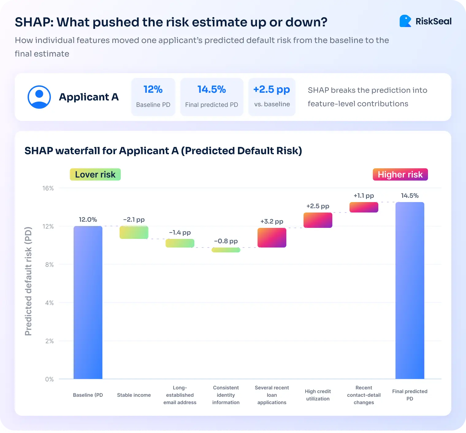
Imagine a model with a baseline default probability of 12%. This is its starting point before considering one applicant’s details.
Several features may reduce the default risk estimate:
Other features may increase it:
Together, these factors produce a final default estimate of 14.5%.
This example simplifies how contributions combine. In practice, SHAP values add up cleanly on the model's internal scale, not always directly in probability terms.
The value lies in the direction and size of each contribution. The team can see which signals lowered risk and which signals outweighed them.
SHAP is useful for individual application reviews. An analyst can identify the strongest drivers behind one result.
It can also support reason-code development. Teams can connect influential variables with approved explanations.
At the portfolio level, SHAP can summarize common feature effects. It may show how model behavior differs between products or customer groups.
A SHAP chart is not automatically a compliant explanation. It describes model influence, not lending policy.
A feature may strongly affect the prediction without being suitable for applicant communication. The lender must still review its relevance.
Raw values also need careful translation. A technical feature name may mean little to an applicant or auditor.
For example, “contact_change_count_90d” may be technically correct. “Recent changes to contact information” is clearer.
Even then, the explanation must reflect the actual decision. It should not mention a feature that had little effect on the result.
SHAP therefore provides evidence, not finished communication. Risk teams must connect that evidence with policy and governance rules.
LIME, or Local Interpretable Model-agnostic Explanations, also explains individual predictions, but it uses a different approach. It examines how the model behaves around one specific case.
The method creates variations of that applicant’s data and observes how the original model responds.
Using those observations, LIME builds a simpler local model that approximates the original model’s behavior within a limited area.
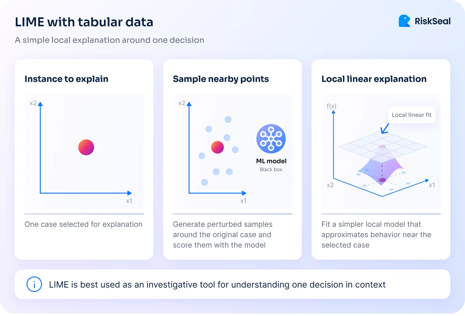
Think of it as a neighborhood map. It helps explain the area around one location, but it does not describe the entire city.
For example, an analyst may investigate why one applicant was rejected.
LIME might show that slightly increasing the applicant’s declared income would not change the outcome, while reducing the number of recent credit inquiries would.
This helps explain how the model behaves around that specific application, even if it says little about the rest of the portfolio.
LIME can also be applied to models that do not have built-in interpretation tools. Its model-agnostic design makes it flexible.
Risk teams may use it to assess whether a decision appears locally sensible and to gain an intuitive view of a complex prediction.
The simplified model remains an approximation. It does not perfectly reproduce the original model.
Results may change depending on the sampling choices used to generate nearby cases. Small changes in the applicant’s data can also produce different explanations.
This does not necessarily mean that one result is wrong. Different methods may use different baselines, assumptions, or definitions of influence.
Still, stability matters in credit risk assessment. Teams should test whether LIME explanations remain reasonably consistent under similar settings.
LIME works best as an investigative tool. It should not serve as the sole justification for a lending decision.
ALE, or Accumulated Local Effects, focuses on broader model behavior. It shows how predictions tend to change as one feature changes.
.webp)
For example, a risk team may examine email age. The question is not about one applicant.
Instead, the team asks how predicted risk changes across the portfolio.
Does risk fall between one month and one year? Does the relationship flatten after several years?
ALE can answer similar questions about debt-to-income ratio. It can show whether risk rises gradually or sharply.
This helps teams identify nonlinear relationships. It also supports checks for expected monotonic behavior.
Credit variables often relate to each other. Income may connect with loan amount, limits, and debt-to-income ratio.
Changing one variable independently may create unrealistic applicants. A very low income paired with a very high credit limit may rarely occur.
ALE tries to stay closer to combinations found in real data. It measures changes within smaller feature intervals.
This makes it useful when correlated variables complicate interpretation. Teams can study effects without moving too far outside observed patterns.
In my work with alternative data, this becomes especially important. Digital signals rarely operate as fully isolated variables.
Email age may relate to account history and platform registrations. Phone stability may connect with device continuity and identity consistency.
ALE can help show whether these relationships remain sensible. It may reveal that one feature matters only within a narrow range.
It can also expose unexpected curves. Risk might fall with email age before becoming stable.
Such findings support model validation and feature review. They can also guide monitoring after deployment.
However, ALE mainly explains population-level behavior. It does not explain one applicant’s full decision.
Its results can become unstable in sparse ranges. One-dimensional plots may also hide interactions between variables.
Most importantly, ALE does not prove causation. It shows how the model behaves, not why the outcome occurs.
Permutation Feature Importance, or PFI, asks a different question. It measures how much model performance depends on each feature.
.webp)
The basic experiment is simple:
A large drop suggests strong model dependence. A small drop suggests limited additional contribution.
Consider this hypothetical result:
PFI can help rank features during development. It also helps teams challenge variables that add complexity without much value.
Lenders can compare PFI results across model versions. They can track whether feature dependence changes over time.
This supports feature selection and monitoring. It may reveal that a model has become too reliant on one signal.
Correlated features create a major limitation. Two variables may contain similar information.
If one gets shuffled, the other may preserve much of the signal. Performance may fall only slightly.
That does not prove the shuffled feature is unimportant. It may only show that another variable can replace it.
Grouped or conditional permutation methods can reduce this problem. Standard PFI results still require contextual review.
PFI also does not explain one applicant’s score. It measures performance dependence across a dataset.
That makes it valuable for global analysis. It should sit beside local methods rather than replace them.
Suppose a model assigns an applicant a relatively high default estimate. The risk team now needs to investigate it.
The workflow might look like this:
These methods may examine the same variables. However, they do not produce interchangeable answers.
SHAP explains what moved a prediction. LIME approximates behavior near that prediction.
ALE examines broader feature effects. PFI measures dependence through performance loss.
Explainability should therefore not become one final chart. It should support different questions throughout the model lifecycle.
Teams may use it during development, validation, approval, monitoring, and investigation. Each stage requires a different view.
Alternative data can strengthen credit risk assessment for thin-file applicants. It adds context beyond previous repayment history.
However, some signals may be less familiar to risk teams. That makes clear interpretation especially important.
A lender may already understand the debt-to-income ratio. Email age or digital identity consistency may require more context.
The first question is whether a signal influenced one score. SHAP or LIME can help answer it.
The next question concerns broader behavior. ALE can show how the model responds across realistic ranges.
PFI can test whether the signal genuinely supports predictive performance. It may also reveal weak or unnecessary variables.
Alternative signals should not become isolated red flags. A single recent email address should not automatically determine an outcome.
The model should consider the wider pattern. Email history, phone stability, device continuity, and identity consistency may provide stronger context together.
Explainability helps risk teams inspect that interaction. It can show whether one signal dominates the model unnecessarily.
It can also reveal when several moderate signals combine. That view is often more useful than a binary warning.
At RiskSeal, we treat explanations as part of useful model output. A score alone does not give teams enough context.
Our aim is to show which digital signals influenced risk. We also indicate whether they pushed the result higher or lower.
That context helps lenders validate the model against their policies. It can also support analyst review and rule development.
I have seen stronger adoption when teams can challenge outputs directly. Explainability reduces uncertainty around unfamiliar data.
It does not remove regulatory responsibility. Instead, it gives teams better evidence for managing that responsibility.
Before using explanations in production, confirm that:
Unexpected explanation changes may indicate drift or data issues. They may also reveal changing model dependence.
Explainability does not make every credit model fully transparent. But at least it gives risk teams better ways to examine complexity.
The real value lies in accurate questions. Is the model learning sensible relationships? Does the explanation match the decision? Can teams review, challenge, and responsibly act on the result?
A useful credit model should provide more than a prediction. It should provide enough evidence to support informed action.
.webp)
Explore how email address analysis can provide alternative data for credit scoring, impacting loan approval rates.

.webp)
Discover how BNPL reshapes lending as split payments boost access and alternative credit scoring helps manage rising credit risk.
.webp)
Discover how reverse phone lookup boosts credit risk scoring—verify identity, detect fraud, and assess solvency with just a phone number.